geoR solution
Paulo Justiniano Ribeiro Jr
Geostatistical analysis with the geoR package
Paulo Justiniano Ribeiro Jr, LEG: Statistics and Geoinformation Lab, DEST: Department of Statistics, UFPR: Federal University of Paraná
- A (very) basic geoR session
- Loading and exploring the data
- Model estimation
- Model prediction
- Bayesian inferance
This is a brief overview of some functionalities in geoR. We refer to the geoR “Tutorials” page http://www.leg.ufpr.br/geoR/tutorials for further examples.
A (very) basic geoR session
## Required package.
require(geoR)
## Loading a data-set included in the package
data(s100)
We first do a quick data display with exploratory checks on spatial patterns, trends in the coordinates, and distribution of the data. We are using the default plot for a geodata object in geoR: plot.geodata. The lowess argument adds a smooth line to the upper right scatter plot (data value vs y value) and to the lower left scatter plot (x value vs data value). The upper left plot shows color coded data quartile at the location of the data
plot(s100, lowess = TRUE)
Another function allows for more options for displaying the data.
points(s100)
args(points.geodata)## function (x, coords = x$coords, data = x$data, data.col = 1,
## borders = x$borders, pt.divide = c("data.proportional", "rank.proportional",
## "quintiles", "quartiles", "deciles", "equal"), lambda = 1,
## trend = "cte", abs.residuals = FALSE, weights.divide = "units.m",
## cex.min, cex.max, cex.var, pch.seq, col.seq, add.to.plot = FALSE,
## x.leg, y.leg = NULL, dig.leg = 2, round.quantiles = FALSE,
## permute = FALSE, ...)
## NULLThe brief summary include information on the distances between data points.
summary(s100)## Number of data points: 100
##
## Coordinates summary
## Coord.X Coord.Y
## min 0.005638006 0.01091027
## max 0.983920544 0.99124979
##
## Distance summary
## min max
## 0.007640962 1.278175109
##
## Data summary
## Min. 1st Qu. Median Mean 3rd Qu. Max.
## -1.1680 0.2730 1.1050 0.9307 1.6100 2.8680
##
## Other elements in the geodata object
## [1] "cov.model" "nugget" "cov.pars" "kappa" "lambda"There are several options for computing the empirical variogram. Here we use default options except for the argument setting the maximum distance (max.dist) to be considered between pairs of points.
s100.v <- variog(s100, max.dist = 1)
plot(s100.v)
Turning to the parameter estimation we fit the model with a constant mean, isotropic exponential correlation function and allowing for estimating the variance of the conditionally independent observations (nugget variance)
(s100.ml <- likfit(s100, ini = c(1, 0.15)))## likfit: estimated model parameters:
## beta tausq sigmasq phi
## "0.7766" "0.0000" "0.7517" "0.1827"
## Practical Range with cor=0.05 for asymptotic range: 0.5473814
##
## likfit: maximised log-likelihood = -83.57summary(s100.ml)## Summary of the parameter estimation
## -----------------------------------
## Estimation method: maximum likelihood
##
## Parameters of the mean component (trend):
## beta
## 0.7766
##
## Parameters of the spatial component:
## correlation function: exponential
## (estimated) variance parameter sigmasq (partial sill) = 0.7517
## (estimated) cor. fct. parameter phi (range parameter) = 0.1827
## anisotropy parameters:
## (fixed) anisotropy angle = 0 ( 0 degrees )
## (fixed) anisotropy ratio = 1
##
## Parameter of the error component:
## (estimated) nugget = 0
##
## Transformation parameter:
## (fixed) Box-Cox parameter = 1 (no transformation)
##
## Practical Range with cor=0.05 for asymptotic range: 0.5473814
##
## Maximised Likelihood:
## log.L n.params AIC BIC
## "-83.57" "4" "175.1" "185.6"
##
## non spatial model:
## log.L n.params AIC BIC
## "-125.8" "2" "255.6" "260.8"
##
## Call:
## likfit(geodata = s100, ini.cov.pars = c(1, 0.15))Finally, we start the spatial prediction defining a grid of points. The kriging function by default performs ordinary kriging. It minimaly requires the data, prediction locations and estimated model parameters.
s100.gr <- expand.grid((0:100)/100, (0:100)/100)
s100.kc <- krige.conv(s100, locations = s100.gr, krige = krige.control(obj.model = s100.ml))
names(s100.kc)
## [1] "predict" "krige.var" "beta.est" "distribution" "message"
## [6] "call"If the locations forms a grid the predictions can be visualised as image, contour or persp plots. Image plots shows the predicted values (left) and the respective std errors.
par(mfrow = c(1, 2), mar = c(3.5, 3.5, 0.5, 0.5))
image(s100.kc, col = gray(seq(1, 0.2, l = 21)))
contour(s100.kc, nlevels = 11, add = TRUE)
image(s100.kc, val = sqrt(krige.var), col = gray(seq(1, 0.2, l = 21)))
It is worth to notice that under the Gaussian model the prediction errors depend on the coordinates of the data, and not on their values (except through model parameter estimates).
image(s100.kc, val = sqrt(krige.var), col = gray(seq(1, 0.2, l = 21)), coords.data = TRUE)
Loading and exploring the data
There are some datasets included in geoR which can be listed as follows. We use some of them to illustrate further options in the functions.
## Datasets included in geoR.
data(package = "geoR")
Some of them are of the class “geodata” which is convenient (but not compulsory!) to use with geoR functions. Others are simply data.frames from which “geodata” can be created. “geodata” (S3) objects are just lists with a class “geodata” and must have elements “coords” and “data”. Optional elements includes “covariates”, “units.m” among others (see help(as.geodata)).
class(s100)## [1] "geodata"class(parana)## [1] "geodata"class(Ksat)## [1] "geodata"class(camg)## [1] "data.frame"head(camg)## east north elevation region ca020 mg020 ctc020 ca2040 mg2040 ctc2040
## 1 5710 4829 6.10 3 52 18 106.0 40 16 86.3
## 2 5727 4875 6.05 3 57 20 131.1 49 21 123.1
## 3 5745 4922 6.30 3 72 22 114.6 63 22 101.7
## 4 5764 4969 6.60 3 74 11 114.4 74 12 95.6
## 5 5781 5015 6.60 3 68 34 124.4 44 36 106.3
## 6 5799 5062 5.75 3 45 27 132.9 27 22 105.3ctc020 <- as.geodata(camg, coords.col = c(1, 2), data.col = 7, covar.col = c(3, 4))The function calls shown above mostly use default options and it is worth examine the arguments (and the help files).
args(plot.geodata)## function (x, coords = x$coords, data = x$data, borders = x$borders,
## trend = "cte", lambda = 1, col.data = 1, weights.divide = "units.m",
## lowess = FALSE, scatter3d = FALSE, density = TRUE, rug = TRUE,
## qt.col, ...)
## NULLargs(points.geodata)## function (x, coords = x$coords, data = x$data, data.col = 1,
## borders = x$borders, pt.divide = c("data.proportional", "rank.proportional",
## "quintiles", "quartiles", "deciles", "equal"), lambda = 1,
## trend = "cte", abs.residuals = FALSE, weights.divide = "units.m",
## cex.min, cex.max, cex.var, pch.seq, col.seq, add.to.plot = FALSE,
## x.leg, y.leg = NULL, dig.leg = 2, round.quantiles = FALSE,
## permute = FALSE, ...)
## NULLargs(variog)## function (geodata, coords = geodata$coords, data = geodata$data,
## uvec = "default", breaks = "default", trend = "cte", lambda = 1,
## option = c("bin", "cloud", "smooth"), estimator.type = c("classical",
## "modulus"), nugget.tolerance, max.dist, pairs.min = 2,
## bin.cloud = FALSE, direction = "omnidirectional", tolerance = pi/8,
## unit.angle = c("radians", "degrees"), angles = FALSE, messages,
## ...)
## NULLWe point in particular to three arguments:
- borders: a matrix with coordinates of a polygon limiting the area
- lambda: parameter of the BoxCox transformation
- trend: a matrix, formula or special words (“1st”, “2nd”) specifying a mean model To find out more about the trend argument, look at trend.spatial
Borders are conveniently dealt with if included in the geodata object. As an example, let us add borders to the s100 data. {r, s100borders, fig.width=5, fig.height=5} s100$borders <- matrix(c(0,0,1,0,1,1,0,1,0,0), ncol=2, byrow=TRUE) points(s100)
If you don’t have the coordinates of the border consider setting them manually by using “locator()” over the “points()” plot.
The dataset Ksat with data on the saturated soil conductivity has a clear asymetric behaviour and the BoxCox transformation suggests to log transform the data.
data(Ksat)
require(MASS)
## Loading required package: MASSsummary(Ksat)## Number of data points: 32
##
## Coordinates summary
## x y
## min 2.5 0.8
## max 21.0 9.1
##
## Distance summary
## min max
## 0.509902 18.552897
##
## Borders summary
## x y
## min 0.0 0
## max 22.5 13
##
## Data summary
## Min. 1st Qu. Median Mean 3rd Qu. Max.
## 0.02000 0.09225 0.30500 0.87210 1.14200 4.30000boxcox(Ksat)
The differences between the exploratory plots are clear.
plot(Ksat, lowess = TRUE)
plot(Ksat, lowess = TRUE, lambda = 0)
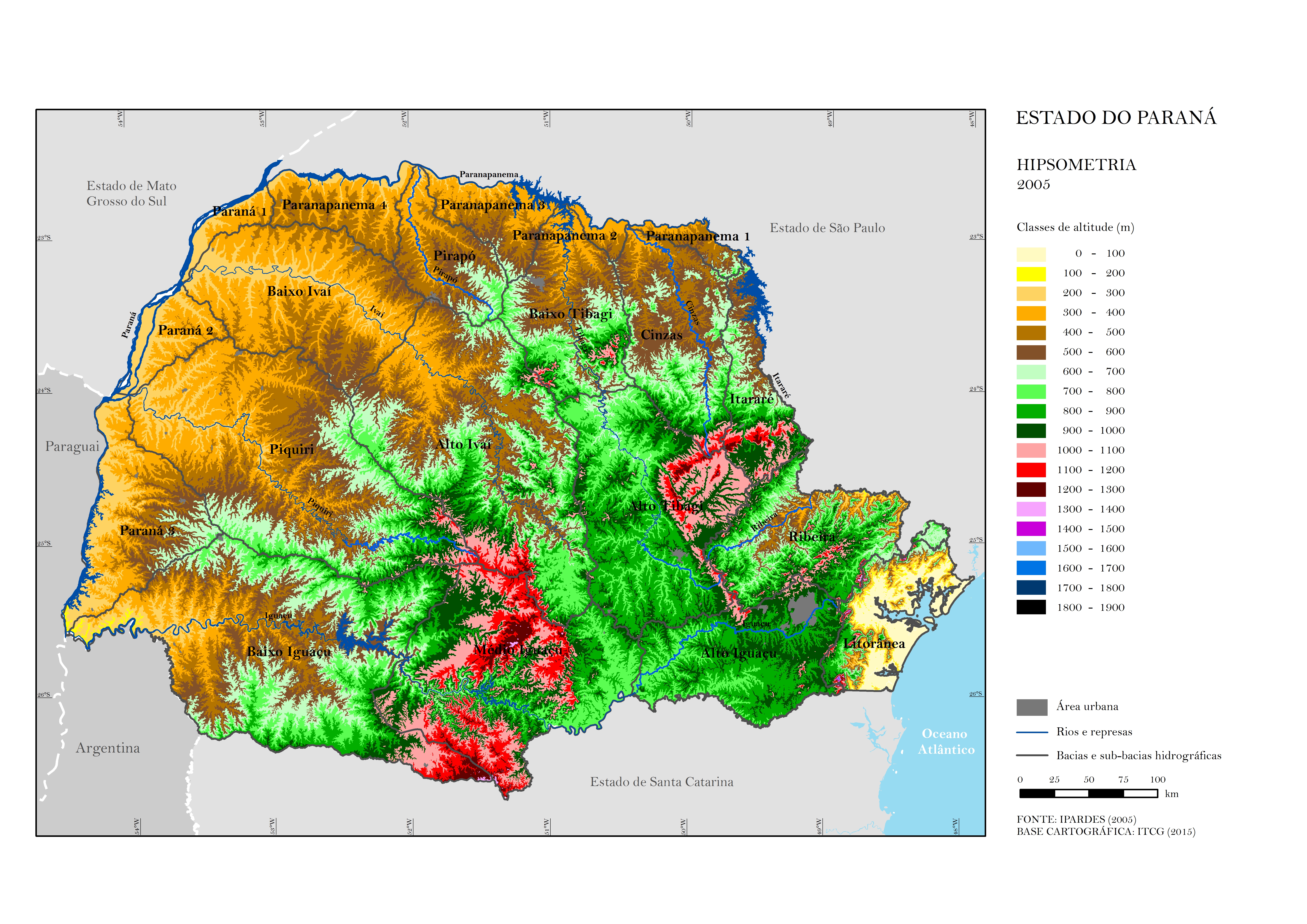
We now use the Paraná rainfall data to illustrate the usage and effect of trend argument. Notice that the data also include the borders of the state. It may be helpful to also have a topographic map of the state.
data(parana)
summary(parana)
## Number of data points: 143
##
## Coordinates summary
## east north
## min 150.1220 70.3600
## max 768.5087 461.9681
##
## Distance summary
## min max
## 1.0000 619.4925
##
## Borders summary
## east north
## min 137.9873 46.7695
## max 798.6256 507.9295
##
## Data summary
## Min. 1st Qu. Median Mean 3rd Qu. Max.
## 162.8 234.2 269.9 274.4 318.2 413.7
##
## Other elements in the geodata object
## [1] "loci.paper"It is clear from the exploratory plot that there is a gradient of the response along the E-W and N-S coordinates.
plot(parana, lowess = TRUE)
If the argument trend is provided an ordinary regression is fitted and the residuals are plotted. The options trend=“1st” defines a linear trend in the coordinates and is equivalent to trend=~coords. More generally a formula on a set of covariates can be used.
plot(parana, trend = "1st", lowess = TRUE)
The effect of the trend on the variogram is very noticeable in this example.
par(mfrow = c(1, 2))
parana.vario <- variog(parana, max.dist = 400)
plot(parana.vario)
parana.variot <- variog(parana, trend = "1st", max.dist = 400)
plot(parana.variot)
Next we show a simple Monte Carlo test using the empirical variogram. The envelope reflects the assumption of no spatial correlation and is given by permutations of the data across the sampling locations.
s100.v <- variog(s100, max.dist = 1)
s100.v.env <- variog.mc.env(s100, obj.variog = s100.v)
plot(s100.v, env = s100.v.env)
To close this section we show a helper function which facilitate building empirical variograms on different directions which may be used to investigate anisotropy. The default directions are 0, 45, 90 and 135 degrees. So to compute the 0 direction variogram, you go through each point and consider only its square distances to points that are between -22.5 and 22.5 degrees from the point considered. Repeat for all points and average.
s100.v4 <- variog4(s100, max.dist = 1)
plot(s100.v4, env = s100.v.env, omni = TRUE)
Question 1:
Investigate the residual spatial structure for the Paraná rainfall data. Is the linear trend sufficient, or do you need a more complicated structure to explain the spatial dependence?
Model estimation
The are four methods for estimating the (covariance) model parameters implemented in geoR.
- visual variogram fitting: using the function eyefit().
- variogram fitting: using the function variofit() basically fitting a nnon-linear model to the empirical variogram.
- likelihood (ML or REML): using the function likfit().
- Bayesian inference: using the function krige.bayes().
We now illustrate the first three, leaving Bayesian inference for later. eyefit() provides an interactive visual model fitting tool which can be used on its own to provide estimates, or to set reasonable initial values for the other methods. Try experimenting with the following.
We leave the eyefit code cunk out of the solution file, since it is interactive
variofit() allows for several options. In what follows we show least squares based variogram fits for the parana data under constant mean and a trend in the coordinates. By default a exponential correlation function (which corresponds to the Matérn model with kappa=0.5) is used. We also show fits for spherical and Matérn (with kappa=1.5) variogram models.
{r, parana-variofit, fig.width=8, fig.height=4} parana.vfit.exp <- variofit(parana.vario) parana.vfit.mat1.5 <- variofit(parana.vario, kappa=1.5) parana.vfit.sph <- variofit(parana.vario, cov.model="sph") parana.vtfit.exp <- variofit(parana.variot) parana.vtfit.mat1.5 <- variofit(parana.variot,kappa=1.5) parana.vtfit.sph <- variofit(parana.variot, cov.model="sph") par(mfrow=c(1,2)) plot(parana.vario) lines(parana.vfit.exp) lines(parana.vfit.mat1.5,col=2) lines(parana.vfit.sph, col=4) plot(parana.variot) lines(parana.vtfit.exp) lines(parana.vtfit.mat1.5, col=2) lines(parana.vtfit.sph, col=4)
Maximum likelihood estimates are obtained by fitting the model to the data (and not to the empirical variogram). Models can be compared by measures of fit, such as the log likelihood.
(parana.ml0 <- likfit(parana, ini = c(4500, 50), nug = 500))## likfit: estimated model parameters:
## beta tausq sigmasq phi
## " 243.4" " 358.5" "9594.1" "1658.6"
## Practical Range with cor=0.05 for asymptotic range: 4968.772
##
## likfit: maximised log-likelihood = -671.6(parana.ml1 <- likfit(parana, trend = "1st", ini = c(1000, 50), nug = 100))## likfit: estimated model parameters:
## beta0 beta1 beta2 tausq sigmasq phi
## "416.4984" " -0.1375" " -0.3997" "385.5180" "785.6904" "184.3863"
## Practical Range with cor=0.05 for asymptotic range: 552.3719
##
## likfit: maximised log-likelihood = -663.9(parana.ml2 <- likfit(parana, trend = "2nd", ini = c(1000, 50), nug = 100))## likfit: estimated model parameters:
## beta0 beta1 beta2 beta3 beta4 beta5 tausq sigmasq
## "423.9282" " 0.0620" " -0.6360" " -0.0004" " 0.0000" " 0.0006" "381.2267" "372.5993"
## phi
## " 77.5441"
## Practical Range with cor=0.05 for asymptotic range: 232.3013
##
## likfit: maximised log-likelihood = -660.2logLik(parana.ml0)## 'log Lik.' -671.6381 (df=4)logLik(parana.ml1)## 'log Lik.' -663.8597 (df=6)logLik(parana.ml2)## 'log Lik.' -660.1756 (df=9)Model prediction
There are two functions for spatial prediction in geoR.
- krige.conv() performing “plug-in” predictions, i.e. treating estimated parameters as if they were the true values
- krige.bayes() for Bayesian inference and prediction
For the former, the function takes: the data, coordinates of the locations, kriging options (through krige.control()) and output options (through output.control()). We use the Paraná rainfall data to illustrate more options for this function. The first step is to define a grid of prediction locations.Note that if your grid is too fine, your computer may choke
parana.gr <- pred_grid(parana$borders, by = 15)
points(parana)
points(parana.gr, pch = 19, col = 2, cex = 0.25)
parana.gr0 <- locations.inside(parana.gr, parana$borders)
points(parana.gr0, pch = 19, col = 4, cex = 0.25)
The following kriging call corresponds to the “universal kriging”. The arguments “trend.d” and “trend.l” require the specification (or terms in a formula) on both, data and prediction locations, respectively. The threshold parameter in output.control is the cutoff for probabilities less than or equal the threshold
args(krige.control)## function (type.krige = "ok", trend.d = "cte", trend.l = "cte",
## obj.model = NULL, beta, cov.model, cov.pars, kappa, nugget,
## micro.scale = 0, dist.epsilon = 1e-10, aniso.pars, lambda)
## NULLargs(output.control)## function (n.posterior, n.predictive, moments, n.back.moments,
## simulations.predictive, mean.var, quantile, threshold, sim.means,
## sim.vars, signal, messages)
## NULLKC <- krige.control(obj.m = parana.ml1, trend.d = "1st", trend.l = "1st")
OC <- output.control(simulations = TRUE, n.pred = 1000, quantile = c(0.1, 0.25, 0.5, 0.75,
0.9), threshold = 350)
parana.kc <- krige.conv(parana, loc = parana.gr, krige = KC, output = OC)
names(parana.kc)## [1] "predict" "krige.var" "beta.est"
## [4] "distribution" "simulations" "mean.simulations"
## [7] "variance.simulations" "quantiles.simulations" "probabilities.simulations"
## [10] "sim.means" ".Random.seed" "message"
## [13] "call"From the output provided we picked the following in the next plot: prediction means, medians, a simulation from the (joint) predictive distribution, and the probability of exceeding the value of 350.
par(mfrow = c(2, 2), mar = c(3, 3, 0.5, 0.5))
image(parana.kc, col = terrain.colors(21), x.leg = c(500, 750), y.leg = c(0, 50))
image(parana.kc, val = parana.kc$quantile[, 3], col = terrain.colors(21), x.leg = c(500, 750),
    y.leg = c(0, 50))
image(parana.kc, val = parana.kc$simulation[, 1], col = terrain.colors(21), x.leg = c(500,
    750), y.leg = c(0, 50))
image(parana.kc, val = 1 - parana.kc$prob, col = terrain.colors(21), x.leg = c(500, 750), y.leg = c(0,
    50))
More generally, simulations can be used to derive maps of quantities of interest. The top panels in next example calls extract minimum and maximum simulated values at each location. The bottom panels shows probabilities of exceeding 300 at each location, and predictive distribution of the proportion of the area exceeding 300.
par(mfrow = c(2, 2), mar = c(3, 3, 0.5, 0.5))
image(parana.kc, val = apply(parana.kc$simulation, 1, min), col = terrain.colors(21), x.leg = c(500,
    750), y.leg = c(0, 50))
image(parana.kc, val = apply(parana.kc$simulation, 1, max), col = terrain.colors(21), x.leg = c(500,
    750), y.leg = c(0, 50))
image(parana.kc, val = apply(parana.kc$simulation, 1, function(x) {
    mean(x > 300, na.rm = T)
}), x.leg = c(500, 750), y.leg = c(0, 50), col = gray(seq(1, 0.2, length = 21)))
hist(apply(parana.kc$simulation, 2, function(x) {
    mean(x > 300, na.rm = T)
}), xlab = "Precip over 300", main = "")
We now pick four particular locations for prediction.
loc4 <- cbind(c(300, 480, 680, 244), c(460, 260, 170, 270))
parana.kc4 <- krige.conv(parana, loc = loc4, krige = KC, output = OC)
points(parana)
points(loc4, col = 2, pch = 19)
par(mfrow = c(1, 4), mar = c(3.5, 3.5, 0.5, 0.5))
apply(parana.kc4$simulation, 1, function(x) {
    hist(x, prob = T, xlim = c(100, 400), ylab = "", main = "")
    lines(density(x))
})
## NULLBayesian Inference
For the Bayesian analysis inference both on model parameters and on spatial predictions (if prediction locations are provided) are performed with a single call to the function krige.bayes(). In the next call we run an analysis setting a discrete prior for the parameter in the (exponential) correlation function and fixing the “nugget” parameter to zero. More general call can set a discrete prior also for the relative nugget through the “tausq.rel” parameter.
args(krige.bayes)## function (geodata, coords = geodata$coords, data = geodata$data,
## locations = "no", borders, model, prior, output)
## NULLparana.bayes <- krige.bayes(parana, loc = parana.gr, model = model.control(trend.d = "1st",
trend.l = "1st"), prior = prior.control(phi.prior = "rec", phi.disc = seq(0, 150, by = 15)),
output = OC)
names(parana.bayes)## [1] "posterior" "predictive" "prior" "model" ".Random.seed"
## [6] "max.dist" "call"names(parana.bayes$posterior)## [1] "beta" "sigmasq" "phi"
## [4] "tausq.rel" "joint.phi.tausq.rel" "sample"par(mfrow = c(1, 1))
plot(parana.bayes)
## parameter `tausq.rel` is fixedFor predictions, the output stored in obj$predictive is similar to that returned by krige.conv() and can be explored and plotted using similar function calls.
names(parana.bayes$predictive)## [1] "mean" "variance" "distribution"
## [4] "simulations" "mean.simulations" "variance.simulations"
## [7] "quantiles.simulations" "probabilities.simulations" "sim.means"par(mfrow = c(1, 3))
image(parana.bayes, col = terrain.colors(21))
image(parana.bayes, val = apply(parana.bayes$pred$simul, 1, quantile, prob = 0.9), col = terrain.colors(21))
hist(apply(parana.bayes$pred$simul, 2, median), main = "")
Question 2
Compare the variability between Bayesian and conventional kriging of the Paraná data set.
How to cite geoR
citation(package = "geoR")##
## To cite package 'geoR' in publications use:
##
## Paulo J. Ribeiro Jr and Peter J. Diggle (2016). geoR: Analysis of
## Geostatistical Data. R package version 1.7-5.2.
## https://CRAN.R-project.org/package=geoR
##
## A BibTeX entry for LaTeX users is
##
## @Manual{,
## title = {geoR: Analysis of Geostatistical Data},
## author = {Paulo J. {Ribeiro Jr} and Peter J. Diggle},
## year = {2016},
## note = {R package version 1.7-5.2},
## url = {https://CRAN.R-project.org/package=geoR},
## }
##
## ATTENTION: This citation information has been auto-generated from the package
## DESCRIPTION file and may need manual editing, see 'help("citation")'.