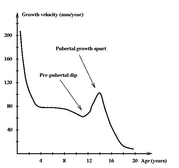
During the years 1955 - 1976 the Children's Hospital in Zurich (Switzerland) conducted a longitudinal study of human growth. Four hundred newly born children were selected, who were then measured and interviewed at regular intervals, half-yearly in early childhood and during puberty, and yearly otherwise, until maturity.
A principal aim of the study was to characterize the ``normal'' growth process, thus providing a baseline for detecting abnormal growth patterns. This is of practical importance, as abnormalities often are indicators for chromosome defects or irregularities in the hormonal system. On the other hand the study provided data for research in endocrinology and developmental psychology.
The main focus of the project was modeling of height growth. The aim was to characterize the sequence of height measurements for each child (36 measurements between birth and 20 years) by a small set of meaningful parameters. Figure 1 shows a typical growth velocity curve. Growth is fast in early childhood and then slows down until the start of the pubertal growth spurt.

Figure 1: Typical human growth velocity curve
There had been a number of previous attempts at this problem, for example by fitting the six parameter double logistic model
h(t) = a1 / (1 + exp (b1 (t-c1))) + a2 / (1 + exp (b2 (t-c2)))
to individual height measurements. The first term is intended to model pre-pubertal growth, whereas the second term accounts for the pubertal growth spurt.
There were two problems with this and other attempts: (1) Lack of fit and (2) a large gender difference in the pre-pubertal parameters a1,b1,c1. The latter casts doubt on the biological meaning of the parameters, as gender differences in pre-pubertal growth are known to be small.
Proposed a biologically more meaningful model for height growth. The reason for the gender difference in the pre-pubertal parameters of the double logistic model is that girls stop growing at a younger age than boys. This in turn is caused by earlier occurrence of puberty in girls. Hormonal changes during puberty not only cause the pubertal growth spurt and full development of primary and secondary sex characteristics but also bone maturation, thereby ``switching off'' growth.
The biological fact that puberty switches off growth suggests a model for growth velocity of the form
v(t) = a1 s1((t - b1) / c1) phi((t - b2) / c2) + a2 s2((t - b2) / c2)
Here s1 and s2 model pre-pubertal growth and the pubertal growth spurt, and phi(x) = 1 - Phi(x) incorporates the ``switch off''. (Phi(x) denotes the cumulative standard gaussian). The incorporation of the switch-off function indeed removes gender differences in a1,b1,c1.
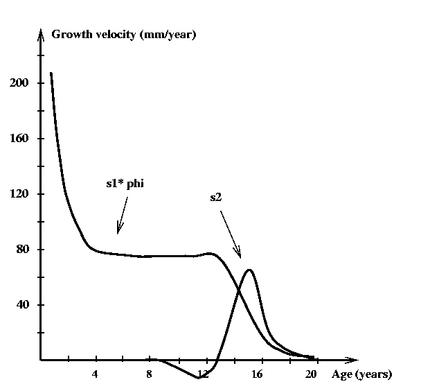
Figure 2: Shape invariant model for growth velocity
Shape-invariant modeling. The idea is to estimate the common component functions s1 and s2, as well as the individual parameters for each child. This approach formalizes the vague notion that ``all children grow alike''. Estimating s1 and s2 was possible because we had data for a sample of children, not just for a single child. Shape invariant modeling had been suggested earlier, but had never been applied to growth curve analysis. Figure 2 shows the components of the shape-invariant model for a typical child. Models for other children differ in amplitude, location, and scale of the components, but the basic shapes are the same.
Shape-invariant modeling of human growth (with R. Largo, Th. Gasser, P.J. Huber, A. Prader). Annals of Human Biology, Vol. 7, No. 6, 1980, pp. 507-528.
Many nonparametric methods in multivariate analysis are based on local averaging. Consider for example the regression problem. The goal of regression is to construct a rule p(x) predicting the value of a response variable Y for given predictor vector x, based on a training sample (y1,x1),...,(yn,xn) of observations for which both response and predictors are known. A standard way of generating such a prediction rule is local averaging:
p(x) = ave (yi | xi in Sr(x)
Here "ave" stands for some kind of average, like the mean or the median, and Sr(x) denotes the sphere around x with radius r.
Local averaging methods work in low dimensions, but in high dimensions they fall victim to the curse of dimensionality: high dimensional samples are always sparse, and the radius of the sphere over which averaging takes place will either have to be large (leading to an estimate with large bias), or the sphere will contain few observations, leading to large variance. There is no general solution to this problem. The best one can hope for is to devise methods able to take advantage of special structure in the data. For example, the association might be linear, or the response might depend on only a few of the predictors.
Formulated the Projection Pursuit paradigm for multivariate modeling:
- Specify initial model
- Repeat
     - Find one-dimensional subspace maximizing deviation between
       data marginal and model marginal
     - Update model to agree with data in this and all previously
       considered marginals
- Until model agrees with data in all marginals.
The key characteristic of Projection Pursuit methods is that they build a high dimensional model from estimates of one-dimensional marginals. They can overcome the curse of dimensionality if a small number of terms suffices.
Applied the Projection Pursuit paradigm to regression, density estimation, and classification. Projection Pursuit regression leads to models of the form
p(x) = sumi si ( ai . x )
where the ai are directions (unit vectors) in predictor space and the si are smooth functions. For example, Projection Pursuit regression applied to a sample generated according to y = x1 * x2 with (x1, x2) ~ U[-1,1]2, constructed a two term model with directions a1 = (0.69, 0.72) and a2 = (-0.63, 0.77), and smooths s1, s2 shown in Figure 3. Note that the procedure essentially uncovers the decomposition x1x2 = 1/4 ((x1+x2)2 - (x1-x2)2).
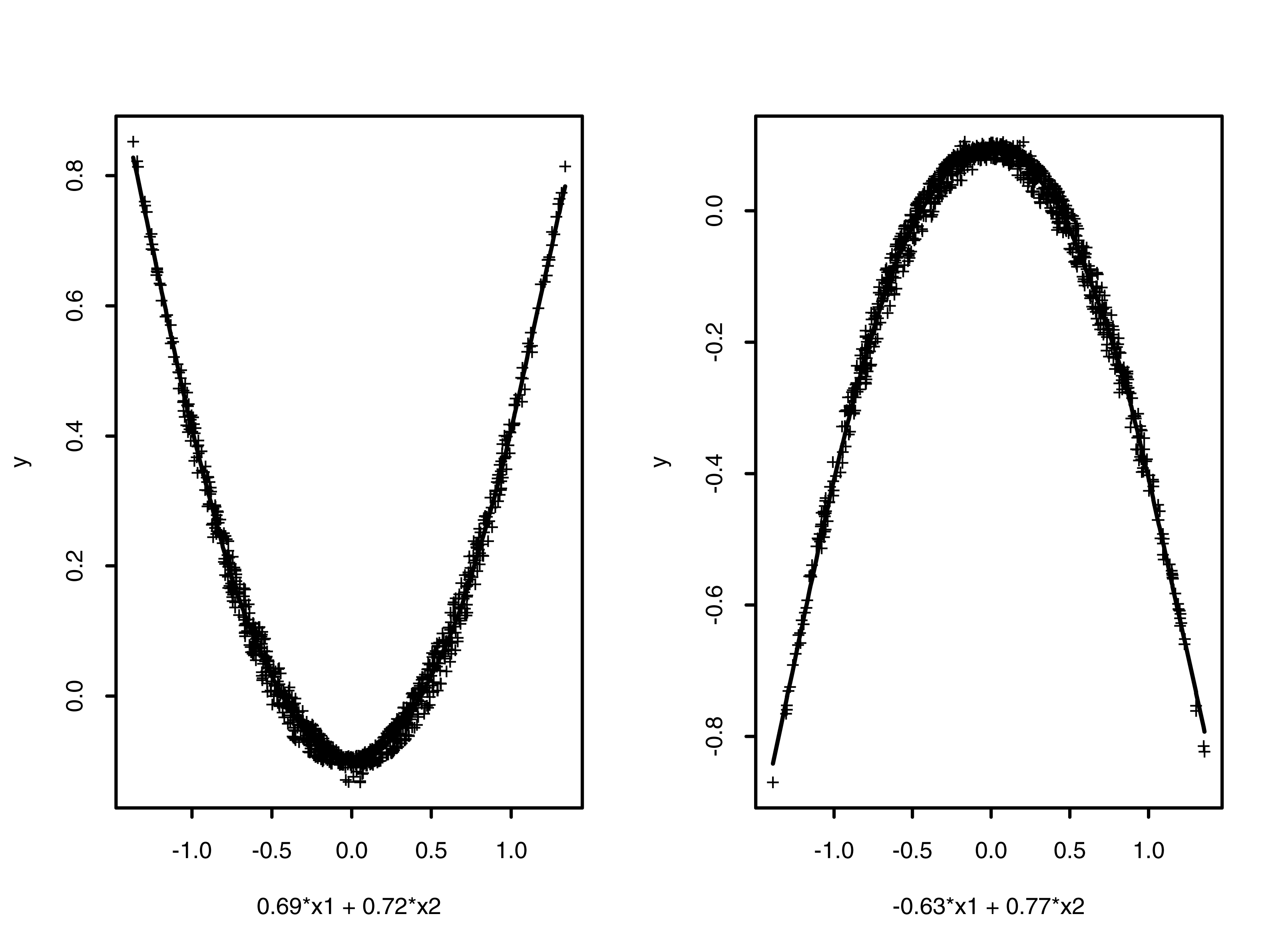
Figure 3: First two terms of Projection Pursuit approximation to y = x1 * x2
Projection Pursuit regression models are similar to Neural Network models, the difference being that in a Neural Network model the functions si are restricted to be shifted and scaled versions of the logistic function. Additive models also are a special case of Projection Pursuit models, with the directions ai restricted to coordinate directions.
Besides regression, classification, and density estimation, the Projection Pursuit paradigm is also applicable to principal component analysis, canonical correlations, and other modeling problems in multivariate analysis.
Projection pursuit regression (with J.H. Friedman). Journal of the American Statistical Association, Vol 76, 1981, pp. 817-823.
Projection pursuit density estimation (with J.H. Friedman, A. Schroeder). Journal of the American Statistical Association, Vol 79, 1984, pp. 599-608.
Extracting information from all but the smallest data sets requires either numerical summaries or graphical presentations. We might summarize a batch of data by the mean and the standard deviation. These two summary statistics will convey an accurate picture of the batch if the data distribution is roughly symmetric and unimodal. If the data is multimodal, on the other hand, the two summary statistics do not accurately reflect the data distribution. In general, numerical summaries are based on assumptions about the data distribution. If these assumptions are violated, the summaries will be misleading. This indicates the need for graphical presentations, which do not make prior assumptions about the data and exploit a human's ability to quickly spot patterns and outliers. Visualization is now widely recognized as an essential component of data analysis.
It is important to recall the state of computer graphics at the time when our work on visualization began. There were no workstations - this concept had not yet been invented. Interactive computing was in its infancy. Bitmapped displays were just appearing. There was little off-the-shelf hardware that could serve as a platform for conducting visualization research. The graphics output device of choice was a Tektronix storage tube display.
Designed, built, and wrote systems software for the Orion-1 workstation, to serve as a platform on which to conduct visualization research. The components of the workstation were a processor board based on a Motorola 68000 microprocessor (one of the early wire wrapped Sun boards, courtesy of Andreas Bechtolsheim, who then went on to found Sun Microsystems), a Lexidata frame buffer, and an IBM 360 emulator for number crunching. Orion-1 had about half the computing power of an IBM 360 mainframe, a bitmap color display, and was dedicated to a single user. While it lacked software infrastructure and was thus hard to program, its performance was far ahead of its time. Two important innovations in data visualization, scatterplot painting (by John McDonald, then a Ph.D student on our project), and the Grand Tour (by Dan Asimov, then a Postdoc on the project), were first implemented and demonstrated on Orion-1.
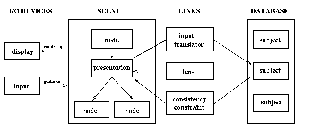
Figure 4: Presentation graphics programming model
Wrote several prototype visualization systems on Symbolics Lisp machines. These systems were based on the concept of presentation graphics (see Figure 4): Icons on the screen (i.e. point symbols in a scatterplot) represent objects (subjects) in a data base. A constraint system enforces consistency between subjects and their visual presentations. Input translators translate gestures directed at presentations into actions on their subjects. Lenses map properties of subjects into their presentations. This system design makes scatterplot painting appear as an obvious operation: Painting changes a the color of an icon on the screen. The constraint system updates the corresponding property of the data objects. This in turn triggers update of all the other graphical presentations of the objects in question. The system design also suggests various extensions, such as painting of histograms, regression trees, and tables, and more general links between data objects and presentations.
Exploring data with the Orion-1 workstation (with J.H. Friedman and J.A. McDonald). Sound film, 25 minutes; Bin-88 Productions, Stanford Linear Accelerator Center, 1982.
Plot windows. Journal of the American Statistical Association, Vol. 82, 1987, pp. 466-475.
Painting multiple views of complex objects (with J.A. McDonald, A. Buja). SIGPLAN Notices, Vol. 10, 1990, pp. 245-257.
Visualization of quantitative data (with A. Buja, J.A. McDonald, J. Michalak, S. Willis). Video tape, 27 minutes; Department of Statistics, University of Washington, 1990.
Variable-resolution bivariate plots. (with C. Huang and J.A.
McDonald.) Journal of Computational and Graphical Statistics, Vol. 6, No. 4, pp 383-396,
1997.
Abstract Compressed
PostScript file PDF file